

What is resolution?
Are you surprised that the very nature of light caps the resolution that we can achieve in microscope images? Luckily, there are workarounds to this limit. These workarounds push the amount of detail in an image by manipulating precisely where and when fluorophores are allowed to emit. As such, they provide us with a completely new set of tools to shrink the distance between two points while still being able to resolve them. But what does “resolving” mean in the first place?
Part one!
The big R that’s actually a tiny d
Resolution is one of those concepts that everyone feels like they understand, but then turns out to be annoyingly muddled. The term itself is used rather indiscriminately to mean different things. There’s image resolution, angular resolution, spectral resolution, and so on. Generally, all these terms reflect the ability to reveal detail in an object, but there are nuanced differences. So, let’s start by stating clearly what this article is about. For light microscopy, resolution is the smallest distance between two points of a specimen that a microscope makes distinguishable. Specifically in the context of fluorescence microscopy, resolution defines a spatial interval between two fluorophores. The closer the two fluorophores can be while remaining discernable in the resulting image, the smaller that distance and thus, the greater the detail resolved. The big R of resolution is actually a tiny d for distance.
So, just how small can d be?
The unfixable blur
First, we need to know what limits resolution. Several components of a microscope contribute to its resolving power. Some of them impact your ability to use resolution. For example, a detector (camera, sensor) with low pixel count will not capture the detail achieved by high resolving power. The opposite is also true. The highest pixel-count camera in the world will not add detail to an image produced by a microscope with low resolution. Similarly, magnification enlarges the image of a specimen, but creating detail lies squarely1 with the microscope’s resolving power.
The truly limiting factors of resolution are the light used to examine a specimen and the ability of a microscope’s optical components to gather and focus that light. There is a simple, insurmountable reason for that dependence: light passing through an objective diffracts. As a result, the image of an emitting fluorophore is blurred, spreading beyond its actual size. As the blurred images of two fluorophores overlap, they become indistinguishable. The larger the blur, the further apart two fluorophores must be to tell them apart. Bingo. That blur, called the point spread function (PSF), restricts the resolution of a light microscope.
1 Caveat: This is one of those muddling instances. Objectives of high magnification often also have high numerical aperture. As we’ll see, resolution is inextricably dependent on numerical aperture. By corollary, there’s a good chance that when you use a high-magnification objective you also increase resolution.
At the limit with Rayleigh, Sparrow, and Abbe
The PSF and its troubling consequences for resolution in optical systems have vexed scientists for centuries. Mathematician and astronomer George Biddell Airy first explained the smeared-out visage of a point of light in 1835. In fact, the PSF of an ideally focused point of light made with a perfect lens is named after him: the Airy pattern, which is a central and bright Airy disc surrounded by dim concentric rings (Figure 1).
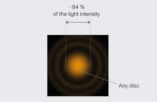
Figure 1.
Airy pattern.
By the turn of the 20th Century, physicists were proclaiming just how close the PSF of two points could get before they become indistinguishable. Three definitions or “limits” stand out. To understand and compare them, it is worth mapping the relative light intensity across the middle of a PSF as projected onto an image plane (Figure 2). The center disc contains the bulk of light intensity (roughly 84 %) while the remainder is distributed in peaks and troughs of decaying amplitude corresponding to the concentric rings that extending out from the center.
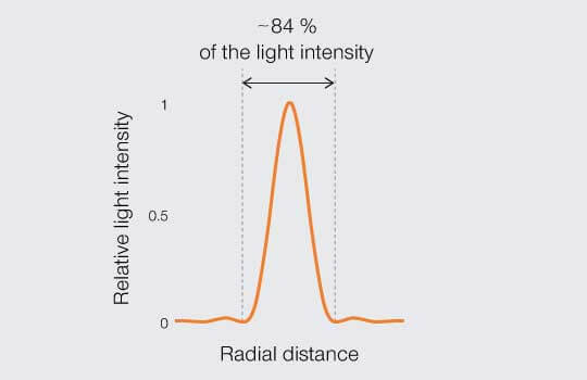
Figure 2.
Intensity profile: distribution of relative light intensity of the point spread function.
The first limit is the Rayleigh criterion. John William Stutt, 3rd Baron Rayleigh, stated that two light points of equal strength are resolved when separated at minimum by the width of the Airy disc (Figure 3A). This spatial interval allows a 20–30% dip in light intensity between the two PSF, which is discernable with the naked eye. A second version of the resolution limit came later from physicist Carroll Mason Sparrow who defined it as the distance at which the light intensity remains constant between the two PSF (Figure 3B). And perhaps the most famous limit is that described by Ernst Abbe who demonstrated that the resolution of any light microscope will never exceed half the wavelength of light (Figure 3C).
Figure 3A.
Rayleigh’s
resolution limit
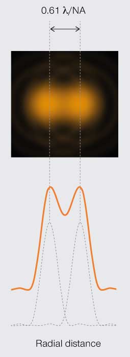
Minimum resolvable separation of two points is the diameter of the central disc in a PSF.
Figure 3B.
Sparrow’s
resolution limit
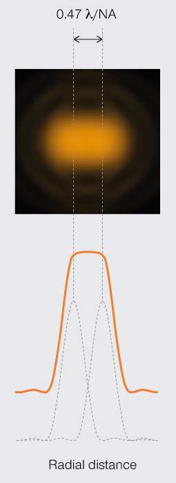
Minimum resolvable separation is when the light intensity plateaus between the two points.
Figure 3C.
Abbe’s
resolution limit
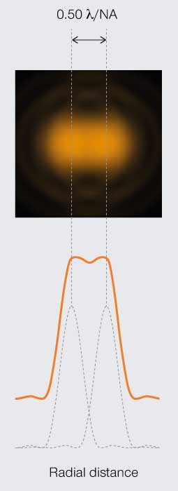
Diffraction limits resolution of a light microscope to about half the wavelength of visible light.
Of apertures and wavelengths
Common to all three definitions for the limit of resolution are two parameters that Abbe identifies in his seminal paper2 as the culprits of diffraction-limited resolution. Abbe was the first to introduce the concept of numerical aperture (NA) – a measure that combines the angle of the cone of light that can enter and leave an objective and the refractive index of the medium in which it operates to characterize its ability to accept and focus light. Abbe explained that the size of a PSF is dictated by the numerical aperture of the microscope objective and the wavelength of light used to image a specimen. Large numerical apertures and high-frequency light produce smaller PSF, which in return shortens the resolvable separation d between two points or fluorophores.
A practical approximation of Abbe’s resolution limit allows empirically measuring the resolution of a fluorescence microscope. If you image a fluorescent bead, you can measure the full width of its PSF central peak at half the maximum intensity (FWHM, Figure 4). Measuring resolution of a microscope is a topic for another article – Voilà.
2 Abbe, E. 1873. Beiträge zur Theorie des Mikroskops und der mikroskopischen Wahrnehmung. Archiv für Mikroskopische Anatomie 9:413–468.
Figure 4.
FWHM resolution
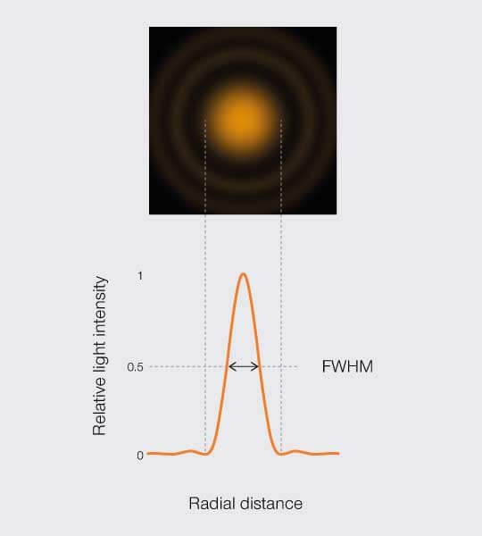
The full width of the PSF at half its maximum is a common estimator for the resolution.
\(d=0.50\frac{\lambda }{\textrm{NA}}\)
So that’s it? d can’t get smaller?
Abbe’s resolution or diffraction limit is fundamentally unassailable. Sure, you could look to use objectives of larger numerical aperture and higher frequency light. But unfortunately, the numerical aperture of modern fluorescence microscopes is at a practical maximum (about 1.4 for oil immersion objectives) and using ultraviolet or x-ray light damages specimens. That means that there is nothing we can do to our microscope system to reduce d any further. But there’s a second player in the generation of an image: the fluorophore. Manipulating the on/off states of fluorophores is another lever we can use to shrink d and thus, a workaround that modifies our approximation of the resolution limit by adding a third parameter.
\(d\approx 0.50\frac{\lambda }{\textrm{NA}}\cdot \textrm{workaround}\)
Stimulated emission depletion (STED) microscopy is one example. In STED, the excitation laser beam used to trigger fluorophore emission is superimposed with a second, donut-shaped de-excitation beam that suppresses that excitation. As a result, only fluorophores at the center of the donut-shaped beam are allowed to fluoresce. Increasing the light intensity of the de-excitation beam constricts the area in which fluorophores are allowed to fluoresce to a substantially smaller diameter than Abbe’s diffraction limit (roughly 200 nm). In this way, fluorophores can be much closer to one another and still be discriminated by the microscope.
The intensity of the de-excitation light is part of the “workaround” parameter here and can be used to approximate the diameter of the narrowed area of fluorescence based on the response of the fluorophores to the de-excitation light. Integrating that approximation into our measure of resolution:
\(d\approx 0.50\frac{\lambda }{\textrm{NA}}\cdot \frac{1}{\sqrt{1+\frac{I}{I_{sat}}}}\)
where Isat is a fluorophore-dependent constant representing the light intensity at which the emission of a fluorophore is reduced by half, and I is the adjustable intensity of the de-excitation beam.3 Increasing I makes the denominator larger and thus, shrinks d. Theoretically, d can become infinitesimally small.
Note that the PSFs of both the excitation and the de-excitation light beams are still diffraction-limited. We cannot make them smaller. However, their interplay with fluorophore states cracks the diffraction barrier.
Another example of this workaround is single-molecule localization microscopy (SMLM). SMLM includes a mechanism that ensures that at any given time, only a few, sparsely distributed, non-overlapping fluorophores of a specimen are in a state where they can fluoresce. A “snapshot” of those fluorophores is made. Then a new subset of fluorophores enters a fluorescent state and another “snapshot” is created. A complete image is constructed from multiple “snapshots”, each of a different random constellation of fluorophores.
Localizing each fluorophore in each snapshot is how the resolution limit is surpassed. The number of photons emitted and detected from a single fluorophore follows a distribution centered on the likely location of the fluorophore. Thus, if enough photons are detected, the likely location of the fluorophore can be narrowed down to an area significantly smaller than the PSF. And there it is: the new “workaround” parameter is the number of emitted photons. Including that likelihood in our measure of resolution looks like this:
\(d\approx 0.50\frac{\lambda }{\textrm{NA}}\cdot \frac{1}{\sqrt{N_{e}}}\)
where Ne is the average number of emitted photons per fluorophore. The more emission photons detected, the larger the denominator and thus, the smaller d becomes. Like with STED, d could theoretically become infinitesimally small.
3 Harke, B. et al. 2008. Resolution scaling in STED microscopy. Opt. Express 16: 4228–4244.
Too much of a good thing
STED and SMLM either shine lots of light on a specimen or capture lots of light from a specimen to manipulate the on/off states of fluorophores and thus, overcome the blur of the PSF. And although both can theoretically improve resolution infinitely, their “workarounds” are precisely what limits their resolving power. MINFLUX, a next-generation superresolution technology that achieves resolution in the single-digit nanometer scale, avoids that limit altogether by completely revamping fluorophore localization. But that too is a topic for another article.